
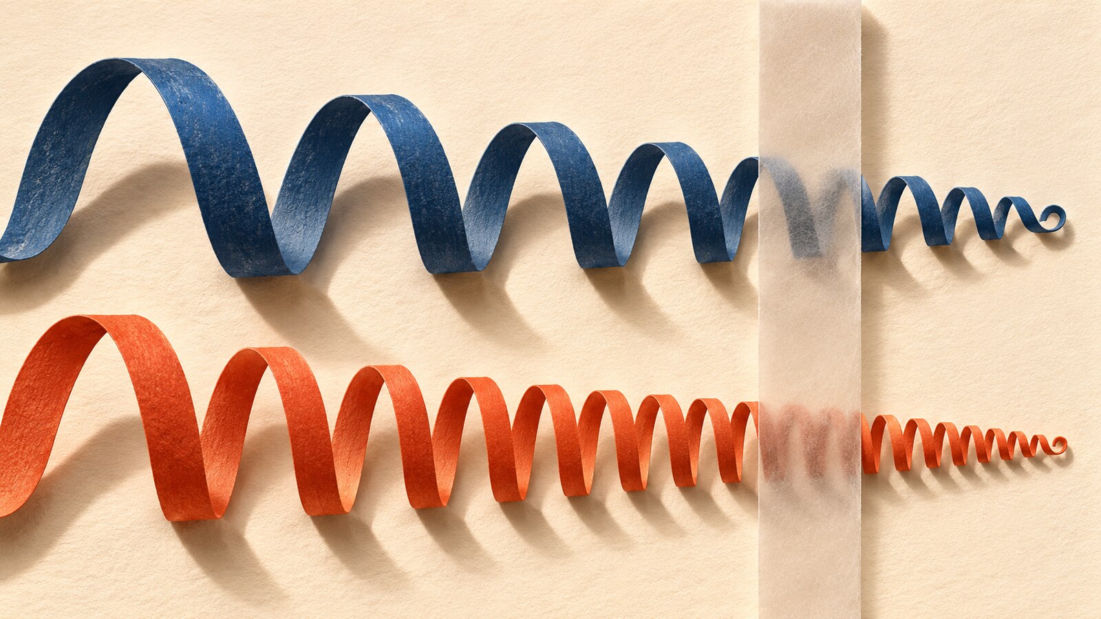
Give two synthetic modes the same positive offset between their endpoints. Fit that shift from their magnitudes and wrapped phases, and the best fit can point backwards. In a two-mode example from the Research Artifact Ledger, the imposed offset is . A least-squares fit using the principal complex logarithm gives about . What happened to the forward shift?
The example starts with a question about black-hole ringdown. A calculation by Ariadna Ribes Metidieri, Béatrice Bonga and Badri Krishnan relates a disturbance at the horizon to its counterpart at null infinity, the idealised far boundary reached by outgoing light. Drawing a different time slice through the spacetime changes which cross-sections of the two boundaries are paired. In their coordinate family, the transfer for each mode therefore picks up a factor that depends on the same real endpoint difference. Source paper, section VI.1, equations (142)–(145)
Where the turns went
In the Ledger example, the first mode advances by radians and the second by . Reading the phase of each complex number returns an angle between and . The first advance now reads as radians and the second as . Both readings locate the correct points on their respective circles. The first has lost one complete turn and the second has lost two. A fit that treats those angles as the full advances produces the apparent disagreement.
There is another piece of information in these particular modes. Each has a known damping rate, so the transfer changes in magnitude as well as phase when the endpoint shifts. For each mode, divide the far-boundary output by the prediction from the unshifted transfer and the matched horizon coefficient . This gives the complex ratio . For the first mode its magnitude is . Taking its ordinary real logarithm and dividing by recovers the only possible offset, . Use that number to predict both complex ratios, keeping their phases as well as their magnitudes. Both predictions agree with the ratios calculated from the constructed coefficients to within . That last number measures rounding in this example.
Why both boundaries matter
The test requires a horizon coefficient and a far-boundary coefficient for each mode, with the transfer between them fixed in advance. Suppose instead that only the far-boundary output is known. Choose an offset, then divide the output by the corresponding transfer to infer a horizon coefficient. When that coefficient is fed back through the transfer, it returns exactly the output you started with. The Ledger script repeats the exercise at offsets of , , and . The same output can accommodate all four.
An independently obtained horizon coefficient would turn that reconstruction into a comparison that could fail. The coefficients would also need to come from the same case, with compatible mode labels, time and frame conventions, rescaling and uncertainties. The example uses invented coefficients and frequencies throughout. It contains no measured horizon data, computed quasinormal frequencies or inference from a detector signal.
The Ledger attributes the transfer law to the source paper and gives the finite test, inputs and verifier separately. AI assisted with the derivation, source mapping, verifier and drafting. An independent AI reviewer checked the source conventions and arithmetic. The example has had no human specialist review or peer review and makes no novelty or priority claim. The featured image is an AI-generated illustration of the two modes. The Ledger assigns no reuse licence. Ledger derivation · Equation-by-equation source map · Reproducible calculation
Loading published comments…